Split Learning—Bank Marketing

The following codes are demos only. It’s NOT for production due to system security concerns, please DO NOT use it directly in production.

In this tutorial, we will use the bank’s marketing model as an example to show how to accomplish split learning in vertical scenarios under the SecretFlow framework. SecretFlow provides a user-friendly Api that makes it easy to apply your Keras model or PyTorch model to split learning scenarios to complete joint modeling tasks for vertical scenarios.

In this tutorial we will show you how to turn your existing ‘Keras’ model into a split learning model under Secretflow to complete federated multi-party modeling tasks.

What is Split Learning？

The core idea of split learning is to split the network structure. Each device (silo) retains only a part of the network structure, and the sub-network structure of all devices is combined together to form a complete network model. In the training process, different devices (silos) only perform forward or reverse calculation on the local network structure, and transfer the calculation results to the next device. Multiple devices complete the training through joint model until convergence.

Alice：have data_alice，model_base_alice

Bob: have data_bob，model_base_bob，model_fuse

1. Alice uses its data to get hidden0 through model_base_Alice and send it to Bob.

2. Bob gets hidden1 with its data through model_base_bob.

3. hidden_0 and hidden_1 are input to the AggLayer for aggregation, and the aggregated hidden_merge is the output.

4. Bob input hidden_merge to model_fuse, get the gradient with label and send it back.

5. The gradient is split into two parts g_0, g_1 through AggLayer, which are sent to Alice and Bob respectively.

6. Then Alice and Bob update their local base net with g_0 or g_1.

Task

Marketing is the banking industry in the ever-changing market environment, to meet the needs of customers, to achieve business objectives of the overall operation and sales activities. In the current environment of big data, data analysis provides a more effective analysis means for the banking industry. Customer demand analysis, understanding of target market trends and more macro market strategies can provide the basis and direction.

The data from kaggle is a set of classic marketing data bank, is a Portuguese bank agency telephone direct marketing activities, The target variable is whether the customer subscribes to deposit product.

Data

1. The total sample size was 11162, including 8929 training set and 2233 test set.

2. Feature dim is 16, target is binary classification.

3. We have cut the data in advance. Alice holds the 4-dimensional basic attribute features, Bob holds the 12-dimensional bank transaction features, and only Alice holds the corresponding label.

Let’s start by looking at what our bank’s marketing data look like?

The original data is divided into Bank Alice and Bank Bob, which stores in Alice and Bob respectively. Here, CSV is the original data that has only been separated without pre-processing, we will use secretflow preprocess for FedData preprocess.

%load_ext autoreload
%autoreload 2

import secretflow as sf
import matplotlib.pyplot as plt

sf.init(['alice', 'bob'], address='local')
alice, bob = sf.PYU('alice'), sf.PYU('bob')

2023-04-27 15:30:12,356 INFO worker.py:1538 -- Started a local Ray instance.

prepare data

import pandas as pd
from secretflow.utils.simulation.datasets import dataset

df = pd.read_csv(dataset('bank_marketing'), sep=';')

We assume that Alice is a new bank, and they only have the basic information of the user and purchased the label of financial products from other bank.

alice_data = df[["age", "job", "marital", "education", "y"]]
alice_data

	age	job	marital	education	y
0	30	unemployed	married	primary	no
1	33	services	married	secondary	no
2	35	management	single	tertiary	no
3	30	management	married	tertiary	no
4	59	blue-collar	married	secondary	no
...	...	...	...	...	...
4516	33	services	married	secondary	no
4517	57	self-employed	married	tertiary	no
4518	57	technician	married	secondary	no
4519	28	blue-collar	married	secondary	no
4520	44	entrepreneur	single	tertiary	no

4521 rows × 5 columns

Bob is an old bank, they have the user’s account balance, house, loan, and recent marketing feedback.

bob_data = df[
    [
        "default",
        "balance",
        "housing",
        "loan",
        "contact",
        "day",
        "month",
        "duration",
        "campaign",
        "pdays",
        "previous",
        "poutcome",
    ]
]
bob_data

	default	balance	housing	loan	contact	day	month	duration	campaign	pdays	previous	poutcome
0	no	1787	no	no	cellular	19	oct	79	1	-1	0	unknown
1	no	4789	yes	yes	cellular	11	may	220	1	339	4	failure
2	no	1350	yes	no	cellular	16	apr	185	1	330	1	failure
3	no	1476	yes	yes	unknown	3	jun	199	4	-1	0	unknown
4	no	0	yes	no	unknown	5	may	226	1	-1	0	unknown
...	...	...	...	...	...	...	...	...	...	...	...	...
4516	no	-333	yes	no	cellular	30	jul	329	5	-1	0	unknown
4517	yes	-3313	yes	yes	unknown	9	may	153	1	-1	0	unknown
4518	no	295	no	no	cellular	19	aug	151	11	-1	0	unknown
4519	no	1137	no	no	cellular	6	feb	129	4	211	3	other
4520	no	1136	yes	yes	cellular	3	apr	345	2	249	7	other

4521 rows × 12 columns

Create Secretflow Environment

Create 2 entities in the Secretflow environment [Alice, Bob]

Where ‘Alice’ and ‘Bob’ are two PYU.

Once you’ve constructed the two objects, you can happily start Splitting Learning.

Import Dependency

from secretflow.data.split import train_test_split
from secretflow.ml.nn import SLModel

Prepare Data

Build Federated Table

Federated table is a virtual concept that cross multiple parties, We define VDataFrame for vertical setting .

1. The data of all parties in a federated table is stored locally and is not allowed to go out of the domain.

2. No one has access to data store except the party that owns the data.

3. Any operation performed on the federated table is scheduled by the driver to each worker, and the execution instructions are delivered layer by layer until the Python runtime of the specific worker. The framework ensures that only the worker with worker.device equal to the Object.device can operate on the data.

4. Federated tables are designed for managing and manipulating multi-party data from a central perspective.

5. Interfaces to Federated Tables are aligned to pandas.DataFrame to reduce the cost of multi-party data operations.

6. The SecretFlow framework provides Plain&Ciphertext hybrid programming capabilities. Vertical federated tables are built using SPU, and MPC-PSI is used to safely get intersection and align data from all parties.

VDataFrame provides read_csv interface similar to pandas, the difference is that secretflow.read_csv receives a dictionary that defines the path of data for both parties. We can use secretflow.vertical.read_csv to build the VDataFrame.

read_csv(file_dict,delimiter,ppu,keys,drop_key)
    filepath: Path of the participant file. The address can be a relative or absolute path to a local file
    spu: SPU Device for PSI; If this parameter is not specified, data must be prealigned
    keys: Key for intersection.

Create spu object

spu = sf.SPU(sf.utils.testing.cluster_def(['alice', 'bob']))

from secretflow.utils.simulation.datasets import load_bank_marketing

# Alice has the first four features,
# while bob has the left features
data = load_bank_marketing(parts={alice: (0, 4), bob: (4, 16)}, axis=1)
# Alice holds the label.
label = load_bank_marketing(parts={alice: (16, 17)}, axis=1)

data is a vertically federated table. It only has the Schema of all the data globally.

Let’s examine the data management of VDF more closely.

As shown in the example, the age field belongs to Alice, so the corresponding column can be obtained from Alice’s partition. However, if Bob tries to obtain the age field, a KeyError error will be reported.

We have a concept called Partition, which is a defined data fragment. Each partition has its own device to which it belongs, and only the device to which it belongs can operate on its data.

data['age'].partitions[alice].data

<secretflow.device.device.pyu.PYUObject at 0x7fd7b1e8cb20>

# You can uncomment this and you will get a KeyError.
# data['age'].partitions[bob]

Next, we perform data preprocessing on the VDataFrame.

We use LabelEncoder and MinMaxScaler as examples. These two preprocessing functions have corresponding concepts in SkLearn, and their usage methods are similar to those in sklearn.

from secretflow.preprocessing.scaler import MinMaxScaler
from secretflow.preprocessing.encoder import LabelEncoder

encoder = LabelEncoder()
data['job'] = encoder.fit_transform(data['job'])
data['marital'] = encoder.fit_transform(data['marital'])
data['education'] = encoder.fit_transform(data['education'])
data['default'] = encoder.fit_transform(data['default'])
data['housing'] = encoder.fit_transform(data['housing'])
data['loan'] = encoder.fit_transform(data['loan'])
data['contact'] = encoder.fit_transform(data['contact'])
data['poutcome'] = encoder.fit_transform(data['poutcome'])
data['month'] = encoder.fit_transform(data['month'])
label = encoder.fit_transform(label)

print(f"label= {type(label)},\ndata = {type(data)}")

label= <class 'secretflow.data.vertical.dataframe.VDataFrame'>,
data = <class 'secretflow.data.vertical.dataframe.VDataFrame'>

Standardize data via MinMaxScaler

scaler = MinMaxScaler()

data = scaler.fit_transform(data)

(_run pid=37133) /Users/zhangxingmeng/miniconda3/envs/secretflow/lib/python3.8/site-packages/sklearn/base.py:443: UserWarning: X has feature names, but MinMaxScaler was fitted without feature names
(_run pid=37133)   warnings.warn(
(_run pid=37133) /Users/zhangxingmeng/miniconda3/envs/secretflow/lib/python3.8/site-packages/sklearn/base.py:443: UserWarning: X has feature names, but MinMaxScaler was fitted without feature names
(_run pid=37133)   warnings.warn(

Next we divide the data set into train-set and test-set.

from secretflow.data.split import train_test_split

random_state = 1234
train_data, test_data = train_test_split(
    data, train_size=0.8, random_state=random_state
)
train_label, test_label = train_test_split(
    label, train_size=0.8, random_state=random_state
)

Summary: At this stage, we have finished defining federated tables, performing data preprocessing, and partitioning the training set and test set. The secretFlow framework defines a set of operations to be built on the federated table (which is the logical counterpart of pandas.DataFrame). The secretflow framework defines a set of operations to be built on the federated table (its logical counterpart is sklearn) Refer to our documentation and API introduction to learn more about other features.

Introduce Model

local version: For this task, a simple DNN can be trained to take in 16-dimensional features, process them through a neural network, and output the probability of positive and negative samples.

Federate version:

• Alice:

  • base_net: Input 4-dimensional feature and go through a DNN network to get hidden.

  • fuse_net: Receive hidden features calculated by Alice and Bob, input them to fusenet for feature fusion, and complete the forward process and backward process.

• Bob:

  • base_net: Input 12-dimensional features, get hidden through a DNN network, and then send hidden to Alice to complete the following operation.

Define Model

Next, we will start creating the federated model.

We have defined the SLTFModel and SLTorchModel, which are used to build split learning for vertically partitioned data. We have also created a simple and easy-to-use extensible interface, allowing you to easily transform your existing model into an SF-Model and perform vertically partitioned federated modeling.

Split learning is to break up a model so that one part is executed locally on the data and the other part is executed on the label side. First let’s define the locally executed model – base_model.

def create_base_model(input_dim, output_dim, name='base_model'):
    # Create model
    def create_model():
        from tensorflow import keras
        from tensorflow.keras import layers
        import tensorflow as tf

        model = keras.Sequential(
            [
                keras.Input(shape=input_dim),
                layers.Dense(100, activation="relu"),
                layers.Dense(output_dim, activation="relu"),
            ]
        )
        # Compile model
        model.summary()
        model.compile(
            loss='binary_crossentropy',
            optimizer='adam',
            metrics=["accuracy", tf.keras.metrics.AUC()],
        )
        return model

    return create_model

We use create_base_model to create their base models for ‘Alice’ and ‘Bob’, respectively.

# prepare model
hidden_size = 64

model_base_alice = create_base_model(4, hidden_size)
model_base_bob = create_base_model(12, hidden_size)

model_base_alice()
model_base_bob()

Model: "sequential"
_________________________________________________________________
 Layer (type)                Output Shape              Param #
=================================================================
 dense (Dense)               (None, 100)               500

 dense_1 (Dense)             (None, 64)                6464

=================================================================
Total params: 6,964
Trainable params: 6,964
Non-trainable params: 0
_________________________________________________________________
Model: "sequential_1"
_________________________________________________________________
 Layer (type)                Output Shape              Param #
=================================================================
 dense_2 (Dense)             (None, 100)               1300

 dense_3 (Dense)             (None, 64)                6464

=================================================================
Total params: 7,764
Trainable params: 7,764
Non-trainable params: 0
_________________________________________________________________

<keras.engine.sequential.Sequential at 0x7fd7a09c31f0>

Next we define the side with the label, or the server-side model – fuse_model In the definition of fuse_model, we need to correctly define loss, optimizer, and metrics. This is compatible with all configurations of your existing Keras model.

def create_fuse_model(input_dim, output_dim, party_nums, name='fuse_model'):
    def create_model():
        from tensorflow import keras
        from tensorflow.keras import layers
        import tensorflow as tf

        # input
        input_layers = []
        for i in range(party_nums):
            input_layers.append(
                keras.Input(
                    input_dim,
                )
            )

        merged_layer = layers.concatenate(input_layers)
        fuse_layer = layers.Dense(64, activation='relu')(merged_layer)
        output = layers.Dense(output_dim, activation='sigmoid')(fuse_layer)

        model = keras.Model(inputs=input_layers, outputs=output)
        model.summary()

        model.compile(
            loss='binary_crossentropy',
            optimizer='adam',
            metrics=["accuracy", tf.keras.metrics.AUC()],
        )
        return model

    return create_model

model_fuse = create_fuse_model(input_dim=hidden_size, party_nums=2, output_dim=1)

model_fuse()

Model: "model"
__________________________________________________________________________________________________
 Layer (type)                   Output Shape         Param #     Connected to
==================================================================================================
 input_3 (InputLayer)           [(None, 64)]         0           []

 input_4 (InputLayer)           [(None, 64)]         0           []

 concatenate (Concatenate)      (None, 128)          0           ['input_3[0][0]',
                                                                  'input_4[0][0]']

 dense_4 (Dense)                (None, 64)           8256        ['concatenate[0][0]']

 dense_5 (Dense)                (None, 1)            65          ['dense_4[0][0]']

==================================================================================================
Total params: 8,321
Trainable params: 8,321
Non-trainable params: 0
__________________________________________________________________________________________________

<keras.engine.functional.Functional at 0x7fd7a0d569d0>

Create Split Learning Model

Secretflow provides the split learning model SLModel.

To initial SLModel only need 3 parameters.

• base_model_dict: A dictionary needs to be passed in all clients participating in the training along with base_model mappings

• device_y: PYU, which device has label

• model_fuse: The fusion model

Define base_model_dict.

base_model_dict:Dict[PYU,model_fn]

base_model_dict = {alice: model_base_alice, bob: model_base_bob}

from secretflow.security.privacy import DPStrategy, LabelDP
from secretflow.security.privacy.mechanism.tensorflow import GaussianEmbeddingDP

# Define DP operations
train_batch_size = 128
gaussian_embedding_dp = GaussianEmbeddingDP(
    noise_multiplier=0.5,
    l2_norm_clip=1.0,
    batch_size=train_batch_size,
    num_samples=train_data.values.partition_shape()[alice][0],
    is_secure_generator=False,
)
label_dp = LabelDP(eps=64.0)
dp_strategy_alice = DPStrategy(label_dp=label_dp)
dp_strategy_bob = DPStrategy(embedding_dp=gaussian_embedding_dp)
dp_strategy_dict = {alice: dp_strategy_alice, bob: dp_strategy_bob}
dp_spent_step_freq = 10

sl_model = SLModel(
    base_model_dict=base_model_dict,
    device_y=alice,
    model_fuse=model_fuse,
    dp_strategy_dict=dp_strategy_dict,
)

INFO:root:Create proxy actor <class 'secretflow.ml.nn.sl.backend.tensorflow.sl_base.PYUSLTFModel'> with party alice.
INFO:root:Create proxy actor <class 'secretflow.ml.nn.sl.backend.tensorflow.sl_base.PYUSLTFModel'> with party bob.

sf.reveal(test_data.partitions[alice].data), sf.reveal(
    test_label.partitions[alice].data
)

(           age       job  marital  education
 1426  0.279412  0.181818      0.5   0.333333
 416   0.176471  0.636364      1.0   0.333333
 3977  0.264706  0.000000      0.5   0.666667
 2291  0.338235  0.000000      0.5   0.333333
 257   0.132353  0.909091      1.0   0.333333
 ...        ...       ...      ...        ...
 1508  0.264706  0.818182      1.0   0.333333
 979   0.544118  0.090909      0.0   0.000000
 3494  0.455882  0.090909      0.5   0.000000
 42    0.485294  0.090909      0.5   0.333333
 1386  0.455882  0.636364      0.5   0.333333

 [905 rows x 4 columns],
       y
 1426  0
 416   0
 3977  0
 2291  0
 257   0
 ...  ..
 1508  0
 979   0
 3494  0
 42    0
 1386  0

 [905 rows x 1 columns])

sf.reveal(train_data.partitions[alice].data), sf.reveal(
    train_label.partitions[alice].data
)

(           age       job  marital  education
 1106  0.235294  0.090909      0.5   0.333333
 1309  0.176471  0.363636      0.5   0.333333
 2140  0.411765  0.272727      1.0   0.666667
 2134  0.573529  0.454545      0.5   0.333333
 960   0.485294  0.818182      0.5   0.333333
 ...        ...       ...      ...        ...
 664   0.397059  0.090909      1.0   0.333333
 3276  0.235294  0.181818      0.5   0.666667
 1318  0.220588  0.818182      0.5   0.333333
 723   0.220588  0.636364      0.5   0.333333
 2863  0.176471  0.363636      1.0   0.666667

 [3616 rows x 4 columns],
       y
 1106  0
 1309  0
 2140  1
 2134  0
 960   0
 ...  ..
 664   0
 3276  0
 1318  0
 723   0
 2863  0

 [3616 rows x 1 columns])

history = sl_model.fit(
    train_data,
    train_label,
    validation_data=(test_data, test_label),
    epochs=10,
    batch_size=train_batch_size,
    shuffle=True,
    verbose=1,
    validation_freq=1,
    dp_spent_step_freq=dp_spent_step_freq,
)

INFO:root:SL Train Params: {'self': <secretflow.ml.nn.sl.sl_model.SLModel object at 0x7fd7a05d8880>, 'x': VDataFrame(partitions={alice: Partition(data=<secretflow.device.device.pyu.PYUObject object at 0x7fd7a05d71c0>), bob: Partition(data=<secretflow.device.device.pyu.PYUObject object at 0x7fd7a05d7af0>)}, aligned=True), 'y': VDataFrame(partitions={alice: Partition(data=<secretflow.device.device.pyu.PYUObject object at 0x7fd7a05d7d00>)}, aligned=True), 'batch_size': 128, 'epochs': 10, 'verbose': 1, 'callbacks': None, 'validation_data': (VDataFrame(partitions={alice: Partition(data=<secretflow.device.device.pyu.PYUObject object at 0x7fd7a05d71f0>), bob: Partition(data=<secretflow.device.device.pyu.PYUObject object at 0x7fd7a05d7820>)}, aligned=True), VDataFrame(partitions={alice: Partition(data=<secretflow.device.device.pyu.PYUObject object at 0x7fd7a05d7280>)}, aligned=True)), 'shuffle': True, 'sample_weight': None, 'validation_freq': 1, 'dp_spent_step_freq': 10, 'dataset_builder': None, 'audit_log_dir': None, 'audit_log_params': {}, 'random_seed': 19860}
E0427 15:30:54.132951000 4559730176 fork_posix.cc:76]                  Other threads are currently calling into gRPC, skipping fork() handlers

(PYUSLTFModel pid=37975) Model: "sequential"
(PYUSLTFModel pid=37975) _________________________________________________________________
(PYUSLTFModel pid=37975)  Layer (type)                Output Shape              Param #
(PYUSLTFModel pid=37975) =================================================================
(PYUSLTFModel pid=37975)  dense (Dense)               (None, 100)               500
(PYUSLTFModel pid=37975)
(PYUSLTFModel pid=37975)  dense_1 (Dense)             (None, 64)                6464
(PYUSLTFModel pid=37975)
(PYUSLTFModel pid=37975) =================================================================
(PYUSLTFModel pid=37975) Total params: 6,964
(PYUSLTFModel pid=37975) Trainable params: 6,964
(PYUSLTFModel pid=37975) Non-trainable params: 0
(PYUSLTFModel pid=37975) _________________________________________________________________
(PYUSLTFModel pid=37975) Model: "model"
(PYUSLTFModel pid=37975) __________________________________________________________________________________________________
(PYUSLTFModel pid=37975)  Layer (type)                   Output Shape         Param #     Connected to
(PYUSLTFModel pid=37975) ==================================================================================================
(PYUSLTFModel pid=37975)  input_2 (InputLayer)           [(None, 64)]         0           []
(PYUSLTFModel pid=37975)
(PYUSLTFModel pid=37975)  input_3 (InputLayer)           [(None, 64)]         0           []
(PYUSLTFModel pid=37975)
(PYUSLTFModel pid=37975)  concatenate (Concatenate)      (None, 128)          0           ['input_2[0][0]',
(PYUSLTFModel pid=37975)                                                                   'input_3[0][0]']
(PYUSLTFModel pid=37975)
(PYUSLTFModel pid=37975)  dense_2 (Dense)                (None, 64)           8256        ['concatenate[0][0]']
(PYUSLTFModel pid=37975)
(PYUSLTFModel pid=37975)  dense_3 (Dense)                (None, 1)            65          ['dense_2[0][0]']
(PYUSLTFModel pid=37975)
(PYUSLTFModel pid=37975) ==================================================================================================
(PYUSLTFModel pid=37975) Total params: 8,321
(PYUSLTFModel pid=37975) Trainable params: 8,321
(PYUSLTFModel pid=37975) Non-trainable params: 0
(PYUSLTFModel pid=37975) __________________________________________________________________________________________________

  0%|                                                                                                                                                                                                 | 0/29 [00:00<?, ?it/s]

(PYUSLTFModel pid=37977) Model: "sequential"
(PYUSLTFModel pid=37977) _________________________________________________________________
(PYUSLTFModel pid=37977)  Layer (type)                Output Shape              Param #
(PYUSLTFModel pid=37977) =================================================================
(PYUSLTFModel pid=37977)  dense (Dense)               (None, 100)               1300
(PYUSLTFModel pid=37977)
(PYUSLTFModel pid=37977)  dense_1 (Dense)             (None, 64)                6464
(PYUSLTFModel pid=37977)
(PYUSLTFModel pid=37977) =================================================================
(PYUSLTFModel pid=37977) Total params: 7,764
(PYUSLTFModel pid=37977) Trainable params: 7,764
(PYUSLTFModel pid=37977) Non-trainable params: 0
(PYUSLTFModel pid=37977) _________________________________________________________________

100%|█| 29/29 [00:02<00:00, 10.18it/s, epoch: 1/10 -  train_loss:0.4129562973976135  train_accuracy:0.8653621673583984  train_auc_1:0.5264993906021118  val_loss:0.40364569425582886  val_accuracy:0.8729282021522522  val_au
100%|█| 29/29 [00:00<00:00, 46.94it/s, epoch: 2/10 -  train_loss:0.35912755131721497  train_accuracy:0.881196141242981  train_auc_1:0.6078442335128784  val_loss:0.36728695034980774  val_accuracy:0.8729282021522522  val_au
100%|█| 29/29 [00:00<00:00, 48.23it/s, epoch: 3/10 -  train_loss:0.32940730452537537  train_accuracy:0.8895474076271057  train_auc_1:0.6757411956787109  val_loss:0.3632793426513672  val_accuracy:0.8729282021522522  val_au
100%|█| 29/29 [00:00<00:00, 46.01it/s, epoch: 4/10 -  train_loss:0.3251654803752899  train_accuracy:0.8821022510528564  train_auc_1:0.7356866598129272  val_loss:0.3409757614135742  val_accuracy:0.8729282021522522  val_auc
100%|█| 29/29 [00:00<00:00, 43.58it/s, epoch: 5/10 -  train_loss:0.28907510638237  train_accuracy:0.8936915993690491  train_auc_1:0.7872641086578369  val_loss:0.32897132635116577  val_accuracy:0.8740331530570984  val_auc_
100%|█| 29/29 [00:00<00:00, 46.98it/s, epoch: 6/10 -  train_loss:0.28495943546295166  train_accuracy:0.8846791982650757  train_auc_1:0.8241945505142212  val_loss:0.31397098302841187  val_accuracy:0.8651933670043945  val_a
100%|█| 29/29 [00:00<00:00, 47.86it/s, epoch: 7/10 -  train_loss:0.26694244146347046  train_accuracy:0.8884698152542114  train_auc_1:0.8525720238685608  val_loss:0.297272264957428  val_accuracy:0.8718231916427612  val_auc
100%|█| 29/29 [00:00<00:00, 49.64it/s, epoch: 8/10 -  train_loss:0.2483515590429306  train_accuracy:0.897090494632721  train_auc_1:0.863089919090271  val_loss:0.3043724000453949  val_accuracy:0.8729282021522522  val_auc_1
100%|█| 29/29 [00:00<00:00, 51.63it/s, epoch: 9/10 -  train_loss:0.25027474761009216  train_accuracy:0.8985066413879395  train_auc_1:0.8572441339492798  val_loss:0.29220494627952576  val_accuracy:0.8751381039619446  val_a
100%|█| 29/29 [00:00<00:00, 57.28it/s, epoch: 10/10 -  train_loss:0.25861650705337524  train_accuracy:0.8927801847457886  train_auc_1:0.8630840182304382  val_loss:0.28584015369415283  val_accuracy:0.8795580267906189  val_

Let’s visualize the training process

# Plot the change of loss during training
plt.plot(history['train_loss'])
plt.plot(history['val_loss'])
plt.title('Model loss')
plt.ylabel('Loss')
plt.xlabel('Epoch')
plt.legend(['Train', 'Val'], loc='upper right')
plt.show()

# Plot the change of accuracy during training
plt.plot(history['train_accuracy'])
plt.plot(history['val_accuracy'])
plt.title('Model accuracy')
plt.ylabel('Accuracy')
plt.xlabel('Epoch')
plt.legend(['Train', 'Val'], loc='upper left')
plt.show()

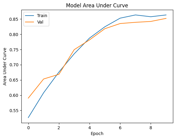
# Plot the Area Under Curve(AUC) of loss during training
plt.plot(history['train_auc_1'])
plt.plot(history['val_auc_1'])
plt.title('Model Area Under Curve')
plt.ylabel('Area Under Curve')
plt.xlabel('Epoch')
plt.legend(['Train', 'Val'], loc='upper left')
plt.show()

Let’s call the evaluation function

global_metric = sl_model.evaluate(test_data, test_label, batch_size=128)

Evaluate Processing:: 100%|█████████████████████████████████████████████████████████████████████████████████████| 8/8 [00:00<00:00, 171.46it/s, loss:0.2899125814437866 accuracy:0.8751381039619446 auc_1:0.8452339172363281]

Compare to local model

Here, we use the same model structure as the one used in the split learning example, but only the model structure for Alice is used in this case. The code for defining the model is shown below.

#### Data

The data also use kaggle’s anti-fraud data. Here, we just use Alice’s data of the new bank.

1. The total sample size was 11162, including 8929 training set and 2233 test set.

2. The feature dimension is 4.

from tensorflow import keras
from tensorflow.keras import layers
import tensorflow as tf
from sklearn.model_selection import train_test_split


def create_model():
    model = keras.Sequential(
        [
            keras.Input(shape=4),
            layers.Dense(100, activation="relu"),
            layers.Dense(64, activation='relu'),
            layers.Dense(64, activation='relu'),
            layers.Dense(1, activation='sigmoid'),
        ]
    )
    model.compile(
        loss='binary_crossentropy',
        optimizer='adam',
        metrics=["accuracy", tf.keras.metrics.AUC()],
    )
    return model


single_model = create_model()

Data process

import pandas as pd
from sklearn.model_selection import train_test_split
from sklearn.preprocessing import MinMaxScaler
from sklearn.preprocessing import LabelEncoder

encoder = LabelEncoder()
single_part_data = alice_data.copy()

single_part_data['job'] = encoder.fit_transform(alice_data['job'])
single_part_data['marital'] = encoder.fit_transform(alice_data['marital'])
single_part_data['education'] = encoder.fit_transform(alice_data['education'])
single_part_data['y'] = encoder.fit_transform(alice_data['y'])

y = single_part_data['y']
alice_data = single_part_data.drop(columns=['y'], inplace=False)

scaler = MinMaxScaler()
alice_data = scaler.fit_transform(alice_data)

train_data, test_data = train_test_split(
    alice_data, train_size=0.8, random_state=random_state
)
train_label, test_label = train_test_split(y, train_size=0.8, random_state=random_state)

alice_data.shape

(4521, 4)

single_model.fit(
    train_data,
    train_label,
    validation_data=(test_data, test_label),
    batch_size=128,
    epochs=10,
    shuffle=False,
)

Epoch 1/10
29/29 [==============================] - 1s 10ms/step - loss: 0.5564 - accuracy: 0.8261 - auc_3: 0.4520 - val_loss: 0.4089 - val_accuracy: 0.8729 - val_auc_3: 0.4384
Epoch 2/10
29/29 [==============================] - 0s 3ms/step - loss: 0.3771 - accuracy: 0.8877 - auc_3: 0.4524 - val_loss: 0.3969 - val_accuracy: 0.8729 - val_auc_3: 0.4322
Epoch 3/10
29/29 [==============================] - 0s 3ms/step - loss: 0.3653 - accuracy: 0.8877 - auc_3: 0.4417 - val_loss: 0.3911 - val_accuracy: 0.8729 - val_auc_3: 0.4316
Epoch 4/10
29/29 [==============================] - 0s 3ms/step - loss: 0.3601 - accuracy: 0.8877 - auc_3: 0.4514 - val_loss: 0.3875 - val_accuracy: 0.8729 - val_auc_3: 0.4443
Epoch 5/10
29/29 [==============================] - 0s 3ms/step - loss: 0.3585 - accuracy: 0.8877 - auc_3: 0.4626 - val_loss: 0.3855 - val_accuracy: 0.8729 - val_auc_3: 0.4680
Epoch 6/10
29/29 [==============================] - 0s 3ms/step - loss: 0.3571 - accuracy: 0.8877 - auc_3: 0.4737 - val_loss: 0.3839 - val_accuracy: 0.8729 - val_auc_3: 0.4867
Epoch 7/10
29/29 [==============================] - 0s 3ms/step - loss: 0.3557 - accuracy: 0.8877 - auc_3: 0.4879 - val_loss: 0.3828 - val_accuracy: 0.8729 - val_auc_3: 0.5052
Epoch 8/10
29/29 [==============================] - 0s 2ms/step - loss: 0.3547 - accuracy: 0.8877 - auc_3: 0.5001 - val_loss: 0.3818 - val_accuracy: 0.8729 - val_auc_3: 0.5164
Epoch 9/10
29/29 [==============================] - 0s 2ms/step - loss: 0.3539 - accuracy: 0.8877 - auc_3: 0.5107 - val_loss: 0.3807 - val_accuracy: 0.8729 - val_auc_3: 0.5290
Epoch 10/10
29/29 [==============================] - 0s 2ms/step - loss: 0.3530 - accuracy: 0.8877 - auc_3: 0.5212 - val_loss: 0.3799 - val_accuracy: 0.8729 - val_auc_3: 0.5368

<keras.callbacks.History at 0x7fd7a85ec7c0>

single_model.evaluate(test_data, test_label, batch_size=128)

8/8 [==============================] - 0s 1ms/step - loss: 0.3799 - accuracy: 0.8729 - auc_3: 0.5368

[0.3799220025539398, 0.8729282021522522, 0.5367639064788818]

Summary

The above two experiments simulate a typical vertical scene training problem. Alice and Bob have the same sample group, but each side has only a part of the features. If Alice only uses her own data to train the model, an accuracy of 0.872, AUC 0.53 model can be obtained. However, if Bob’s data are combined, a model with an accuracy of 0.875 and AUC 0.885 can be obtained.

Conclusion

• This tutorial introduces what is split learning and how to do it in secretFlow.

• It can be seen from the experimental data that split learning has significant advantages in expanding sample dimension and improving model effect through joint multi-party training.

• This tutorial uses plaintext aggregation to demonstrate, without considering the leakage problem of hidden layer. Secretflow provides AggLayer to avoid the leakage problem of hidden layer plaintext transmission through MPC,TEE,HE, and DP. If you are interested, please refer to relevant documents.

• Next, you may want to try different data sets, you need to vertically shard the data first and then follow the flow of this tutorial.