拆分学习：银行营销#

以下代码仅作为演示用，请勿直接在生产环境使用。

在这个教程中，我们将以银行的市场营销模型为例，展示在 SecretFlow 框架下如何完成垂直场景下的拆分学习。 SecretFlow 框架提供了一套用户友好的API，可以很方便的将您的Keras模型或者PyTorch模型应用到拆分学习场景，以完成垂直场景的联合建模任务.

在接下来的教程中我们将手把手演示，如何将您已有的 Keras 模型变成 SecretFlow 下的拆分学习模型，完成联邦多方建模任务。

什么是拆分学习？#

拆分学习的核心思想是将网络结构进行拆分，每个设备（机构）只保留一部分网络结构，所有设备的子网络结构组合在一起，构成一个完整的网络模型。在训练过程中，不同的设备（机构）只对本地的网络结构进行前向或反向计算，并将计算结果传递给下一个设备，多个设备端通过联合模型，完成训练，直到收敛为止。

Alice ：拥有 data_alice ， model_base_alice

Bob ：拥有 data_bob ， model_base_bob ， model_fuse

Alice 用本方的数据通过 model_base_alice 得到 hidden0 ，发送给Bob
Bob 用本方的数据通过 model_base_bob 得到 hidden1
hidden_0 和 hidden_1 输入到 AggLayer 进行聚合，聚合后的 `hidden_merge`为输出
Bob 方输入 hidden_merge 到 model_fuse，结合`label` 得到梯度，并进行回传
通过 AggLayer 将梯度拆分为 g0 , g1 两部分，将 g0 和 g1 分别发送给 Alice 和 Bob
Alice 和 Bob 的 basenet 分别根据 g0 和 g1 对本方的基础模型进行更新

任务#

市场营销是银行业在不断变化的市场环境中，为满足客户需要、实现经营目标的整体性经营和销售的活动。在目前大数据的环境下，数据分析为银行业提供了更有效的分析手段。对客户需求分析，了解目标市场趋势以及更宏观的市场策略都可以提供依据与方向。

数据来自 kaggle 上的经典银行营销数据集，是一家葡萄牙银行机构电话直销的活动，目标变量是客户是否订阅存款产品。

数据#

样本量总计11162个，其中训练集8929，测试集2233
特征16维，标签为2分类
我们预先对数据进行了切割，alice持有其中的4维基础属性特征，bob持有12维银行交易特征，对应的label只有alice方持有

我们先来看看我们的银行市场营销数据长什么样的?

原始数据被拆分为bank_alice和bank_bob，分别存在alice和bob两方。这里的csv是仅经过拆分没有做预处理的原始数据，我们将使用secretflow preprocess进行FedData预处理。

[1]:

%load_ext autoreload
%autoreload 2

import secretflow as sf
import matplotlib.pyplot as plt

sf.init(['alice', 'bob'], address='local')
alice, bob = sf.PYU('alice'), sf.PYU('bob')

2023-04-27 15:30:12,356 INFO worker.py:1538 -- Started a local Ray instance.

数据准备#

[2]:

import pandas as pd
from secretflow.utils.simulation.datasets import dataset

df = pd.read_csv(dataset('bank_marketing'), sep=';')

我们假设Alice是一个新银行，他们只有用户的基本信息，和是否从其他银行购买过理财产品的label

[3]:

alice_data = df[["age", "job", "marital", "education", "y"]]
alice_data

[3]:

	age	job	marital	education	y
0	30	unemployed	married	primary	no
1	33	services	married	secondary	no
2	35	management	single	tertiary	no
3	30	management	married	tertiary	no
4	59	blue-collar	married	secondary	no
...	...	...	...	...	...
4516	33	services	married	secondary	no
4517	57	self-employed	married	tertiary	no
4518	57	technician	married	secondary	no
4519	28	blue-collar	married	secondary	no
4520	44	entrepreneur	single	tertiary	no

4521 rows × 5 columns

Bob端是一个老银行，他们有用户的账户余额，是否有房，是否有贷款，以及最近的营销反馈

[4]:

bob_data = df[
    [
        "default",
        "balance",
        "housing",
        "loan",
        "contact",
        "day",
        "month",
        "duration",
        "campaign",
        "pdays",
        "previous",
        "poutcome",
    ]
]
bob_data

[4]:

	default	balance	housing	loan	contact	day	month	duration	campaign	pdays	previous	poutcome
0	no	1787	no	no	cellular	19	oct	79	1	-1	0	unknown
1	no	4789	yes	yes	cellular	11	may	220	1	339	4	failure
2	no	1350	yes	no	cellular	16	apr	185	1	330	1	failure
3	no	1476	yes	yes	unknown	3	jun	199	4	-1	0	unknown
4	no	0	yes	no	unknown	5	may	226	1	-1	0	unknown
...	...	...	...	...	...	...	...	...	...	...	...	...
4516	no	-333	yes	no	cellular	30	jul	329	5	-1	0	unknown
4517	yes	-3313	yes	yes	unknown	9	may	153	1	-1	0	unknown
4518	no	295	no	no	cellular	19	aug	151	11	-1	0	unknown
4519	no	1137	no	no	cellular	6	feb	129	4	211	3	other
4520	no	1136	yes	yes	cellular	3	apr	345	2	249	7	other

4521 rows × 12 columns

环境的搭建#

环境的搭建
Alice 和 bob 是两个 PYU 。
在 Secretflow 环境中创建 2 个实体 [Alice, Bob]，其中 ‘Alice’ 和 ‘Bob’ 是两个 PYU。 一旦您构建了这两个对象，您可以愉快地开始拆分学习

引入依赖#

[5]:

from secretflow.data.split import train_test_split
from secretflow.ml.nn import SLModel

准备数据#

创建联邦表

联邦表是一个跨多方的虚拟概念，我们定义 VDataFrame 用于垂直场景设置。

联邦表中各方的数据存储在本地，不允许出域。
除了拥有数据的一方之外，没有人可以访问数据存储。
联邦表的任何操作都会由driver调度给每个worker，执行指令会逐层传递，直到特定worker的Python Runtime。框架确保只有当worker的 worker.device 和 Object.device 相同时，才能够操作数据。
联邦表旨在从中心角度管理和操作多方数据。
Federated Table 的接口与 pandas.DataFrame 对齐，以降低多方数据操作的成本。
SecretFlow 框架提供 Plain&Ciphertext （明密文）混合编程能力。垂直联邦表是使用 SPU 构建的， MPC-PSI 用于安全地获取来自各方的交集和对齐数据。

VDataFrame 提供类似于 pandas 的 read_csv 接口，不同之处在于secretflow.read_csv 接收一个定义双方数据路径的字典。我们可以使用 secretflow.vertical.read_csv 来构建 VDataFrame 。

read_csv(file_dict,delimiter,ppu,keys,drop_key)
    filepath: Path of the participant file. The address can be a relative or absolute path to a local file
    spu: SPU Device for PSI; If this parameter is not specified, data must be prealigned
    keys: Key for intersection.

创建spu 对象

[6]:

spu = sf.SPU(sf.utils.testing.cluster_def(['alice', 'bob']))

[7]:

from secretflow.utils.simulation.datasets import load_bank_marketing

# Alice has the first four features,
# while bob has the left features
data = load_bank_marketing(parts={alice: (0, 4), bob: (4, 16)}, axis=1)
# Alice holds the label.
label = load_bank_marketing(parts={alice: (16, 17)}, axis=1)

data 为构建好的垂直联邦表，它从全局上只拥有所有数据的 Schema

我们进一步来看一下VDF的数据管理

通过一个实例可以看出，age这个字段是属于alice的，所以在alice方的partition可以得到对应的列，但是bob方想要去获取age的时候会报`KeyError`错误。

这里有一个Partition的概念，是我们定义的一个数据分片，每个Partition都会有自己的device归属，只有归属的device才可以操作数据。

[8]:

data['age'].partitions[alice].data

[8]:

<secretflow.device.device.pyu.PYUObject at 0x7fd7b1e8cb20>

[ ]:

# You can uncomment this and you will get a KeyError.
# data['age'].partitions[bob]

我们接着对生成的联邦表做数据预处理。

我们这里以LabelEncoder和MinMaxScaler为例，这两个预处理函数在`sklearn`中有对应的概念，它们的使用方法和sklearn中是类似的

[9]:

from secretflow.preprocessing.scaler import MinMaxScaler
from secretflow.preprocessing.encoder import LabelEncoder

[10]:

encoder = LabelEncoder()
data['job'] = encoder.fit_transform(data['job'])
data['marital'] = encoder.fit_transform(data['marital'])
data['education'] = encoder.fit_transform(data['education'])
data['default'] = encoder.fit_transform(data['default'])
data['housing'] = encoder.fit_transform(data['housing'])
data['loan'] = encoder.fit_transform(data['loan'])
data['contact'] = encoder.fit_transform(data['contact'])
data['poutcome'] = encoder.fit_transform(data['poutcome'])
data['month'] = encoder.fit_transform(data['month'])
label = encoder.fit_transform(label)

[11]:

print(f"label= {type(label)},\ndata = {type(data)}")

label= <class 'secretflow.data.vertical.dataframe.VDataFrame'>,
data = <class 'secretflow.data.vertical.dataframe.VDataFrame'>

通过MinMaxScaler做数据标准化

[12]:

scaler = MinMaxScaler()

data = scaler.fit_transform(data)

(_run pid=37133) /Users/zhangxingmeng/miniconda3/envs/secretflow/lib/python3.8/site-packages/sklearn/base.py:443: UserWarning: X has feature names, but MinMaxScaler was fitted without feature names
(_run pid=37133)   warnings.warn(
(_run pid=37133) /Users/zhangxingmeng/miniconda3/envs/secretflow/lib/python3.8/site-packages/sklearn/base.py:443: UserWarning: X has feature names, but MinMaxScaler was fitted without feature names
(_run pid=37133)   warnings.warn(

接着我们将数据集划分成训练集（train-set）和测试集（test-set）

[13]:

from secretflow.data.split import train_test_split

random_state = 1234
train_data, test_data = train_test_split(
    data, train_size=0.8, random_state=random_state
)
train_label, test_label = train_test_split(
    label, train_size=0.8, random_state=random_state
)

小结：到这里为止，我们就完成了联邦表的定义，数据的预处理，以及训练集和测试集的划分。 SecretFlow框架定义了跨越多方的联邦表概念，同时定义了一套构建在联邦表上的操作（它在逻辑上对等 pandas.DataFrame），同时定义了对于联邦表的预处理操作（它在逻辑上对等 sklearn），您在使用过程中遇到问题，可以参考我们的文档以及API介绍，进一步了解其他的功能

模型介绍#

单机版本：”对于该任务一个基本的DNN就可以完成，输入16维特征，经过一个DNN网络，输出对于正负样本的概率。”

创建联邦表

Alice:
- base_net:输入4维特征，经过一个dnn网络得到hidden.
- fuse_net:接收_alice,以及bob计算得到的hidden特征，输入这些特征到fuse_net，进行特征融合，送入之后的网络完成整个前向传播过程和反向传播过程。
Bob:
- base_net:输入12维特征，经过一个dnn网络得到hidden，然后将hidden发送给alice方，完成接下来的运算。

定义模型#

接下来，我们开始创建联邦模型。

接下来我们开始创建我们定义的联邦模型 SLTFModel 和 SLTorchModel(WIP，工作正在进行) ,用于构建垂直场景的拆分学习，我们定义了简单易用的可扩展接口，可以很方便的将您已有的模型，转换成SF—Model，进而进行垂直场景联邦建模。

拆分学习即将一个模型拆分开来，一部分放在数据的本地执行，另外一部分放在有label的一方。首先我们来定义本地执行的模型——base_model

[14]:

def create_base_model(input_dim, output_dim, name='base_model'):
    # Create model
    def create_model():
        from tensorflow import keras
        from tensorflow.keras import layers
        import tensorflow as tf

        model = keras.Sequential(
            [
                keras.Input(shape=input_dim),
                layers.Dense(100, activation="relu"),
                layers.Dense(output_dim, activation="relu"),
            ]
        )
        # Compile model
        model.summary()
        model.compile(
            loss='binary_crossentropy',
            optimizer='adam',
            metrics=["accuracy", tf.keras.metrics.AUC()],
        )
        return model

    return create_model

我们使用create_base_model分别为 Alice 和 Bob 创建他们的base model

[15]:

# prepare model
hidden_size = 64

model_base_alice = create_base_model(4, hidden_size)
model_base_bob = create_base_model(12, hidden_size)

[16]:

model_base_alice()
model_base_bob()

Model: "sequential"
_________________________________________________________________
 Layer (type)                Output Shape              Param #
=================================================================
 dense (Dense)               (None, 100)               500

 dense_1 (Dense)             (None, 64)                6464

=================================================================
Total params: 6,964
Trainable params: 6,964
Non-trainable params: 0
_________________________________________________________________
Model: "sequential_1"
_________________________________________________________________
 Layer (type)                Output Shape              Param #
=================================================================
 dense_2 (Dense)             (None, 100)               1300

 dense_3 (Dense)             (None, 64)                6464

=================================================================
Total params: 7,764
Trainable params: 7,764
Non-trainable params: 0
_________________________________________________________________

[16]:

<keras.engine.sequential.Sequential at 0x7fd7a09c31f0>

接下来我们定义有label的一方，或者server端的模型——fuse_model。在fuse_model的定义中，我们需要正确的定义loss，optimizer，metrics。这里可以兼容所有您已有的Keras模型的配置

[17]:

def create_fuse_model(input_dim, output_dim, party_nums, name='fuse_model'):
    def create_model():
        from tensorflow import keras
        from tensorflow.keras import layers
        import tensorflow as tf

        # input
        input_layers = []
        for i in range(party_nums):
            input_layers.append(
                keras.Input(
                    input_dim,
                )
            )

        merged_layer = layers.concatenate(input_layers)
        fuse_layer = layers.Dense(64, activation='relu')(merged_layer)
        output = layers.Dense(output_dim, activation='sigmoid')(fuse_layer)

        model = keras.Model(inputs=input_layers, outputs=output)
        model.summary()

        model.compile(
            loss='binary_crossentropy',
            optimizer='adam',
            metrics=["accuracy", tf.keras.metrics.AUC()],
        )
        return model

    return create_model

[18]:

model_fuse = create_fuse_model(input_dim=hidden_size, party_nums=2, output_dim=1)

[19]:

model_fuse()

Model: "model"
__________________________________________________________________________________________________
 Layer (type)                   Output Shape         Param #     Connected to
==================================================================================================
 input_3 (InputLayer)           [(None, 64)]         0           []

 input_4 (InputLayer)           [(None, 64)]         0           []

 concatenate (Concatenate)      (None, 128)          0           ['input_3[0][0]',
                                                                  'input_4[0][0]']

 dense_4 (Dense)                (None, 64)           8256        ['concatenate[0][0]']

 dense_5 (Dense)                (None, 1)            65          ['dense_4[0][0]']

==================================================================================================
Total params: 8,321
Trainable params: 8,321
Non-trainable params: 0
__________________________________________________________________________________________________

[19]:

<keras.engine.functional.Functional at 0x7fd7a0d569d0>

创建拆分学习模型#

创建拆分学习模型

我们需要三个参数来初始化SLModel

base_model_dict：一个字典，它需要传入参与训练的所有client以及base_model映射。
device_y：PYU对象，哪一方持有label
model_fuse：融合模型，具体的优化器以及损失函数都在这个模型中进行定义

定义 base_model_dict

base_model_dict:Dict[PYU,model_fn]

[20]:

base_model_dict = {alice: model_base_alice, bob: model_base_bob}

[21]:

from secretflow.security.privacy import DPStrategy, LabelDP
from secretflow.security.privacy.mechanism.tensorflow import GaussianEmbeddingDP

# Define DP operations
train_batch_size = 128
gaussian_embedding_dp = GaussianEmbeddingDP(
    noise_multiplier=0.5,
    l2_norm_clip=1.0,
    batch_size=train_batch_size,
    num_samples=train_data.values.partition_shape()[alice][0],
    is_secure_generator=False,
)
label_dp = LabelDP(eps=64.0)
dp_strategy_alice = DPStrategy(label_dp=label_dp)
dp_strategy_bob = DPStrategy(embedding_dp=gaussian_embedding_dp)
dp_strategy_dict = {alice: dp_strategy_alice, bob: dp_strategy_bob}
dp_spent_step_freq = 10

[22]:

sl_model = SLModel(
    base_model_dict=base_model_dict,
    device_y=alice,
    model_fuse=model_fuse,
    dp_strategy_dict=dp_strategy_dict,
)

INFO:root:Create proxy actor <class 'secretflow.ml.nn.sl.backend.tensorflow.sl_base.PYUSLTFModel'> with party alice.
INFO:root:Create proxy actor <class 'secretflow.ml.nn.sl.backend.tensorflow.sl_base.PYUSLTFModel'> with party bob.

[23]:

sf.reveal(test_data.partitions[alice].data), sf.reveal(
    test_label.partitions[alice].data
)

[23]:

(           age       job  marital  education
 1426  0.279412  0.181818      0.5   0.333333
 416   0.176471  0.636364      1.0   0.333333
 3977  0.264706  0.000000      0.5   0.666667
 2291  0.338235  0.000000      0.5   0.333333
 257   0.132353  0.909091      1.0   0.333333
 ...        ...       ...      ...        ...
 1508  0.264706  0.818182      1.0   0.333333
 979   0.544118  0.090909      0.0   0.000000
 3494  0.455882  0.090909      0.5   0.000000
 42    0.485294  0.090909      0.5   0.333333
 1386  0.455882  0.636364      0.5   0.333333

 [905 rows x 4 columns],
       y
 1426  0
 416   0
 3977  0
 2291  0
 257   0
 ...  ..
 1508  0
 979   0
 3494  0
 42    0
 1386  0

 [905 rows x 1 columns])

[24]:

sf.reveal(train_data.partitions[alice].data), sf.reveal(
    train_label.partitions[alice].data
)

[24]:

(           age       job  marital  education
 1106  0.235294  0.090909      0.5   0.333333
 1309  0.176471  0.363636      0.5   0.333333
 2140  0.411765  0.272727      1.0   0.666667
 2134  0.573529  0.454545      0.5   0.333333
 960   0.485294  0.818182      0.5   0.333333
 ...        ...       ...      ...        ...
 664   0.397059  0.090909      1.0   0.333333
 3276  0.235294  0.181818      0.5   0.666667
 1318  0.220588  0.818182      0.5   0.333333
 723   0.220588  0.636364      0.5   0.333333
 2863  0.176471  0.363636      1.0   0.666667

 [3616 rows x 4 columns],
       y
 1106  0
 1309  0
 2140  1
 2134  0
 960   0
 ...  ..
 664   0
 3276  0
 1318  0
 723   0
 2863  0

 [3616 rows x 1 columns])

[25]:

history = sl_model.fit(
    train_data,
    train_label,
    validation_data=(test_data, test_label),
    epochs=10,
    batch_size=train_batch_size,
    shuffle=True,
    verbose=1,
    validation_freq=1,
    dp_spent_step_freq=dp_spent_step_freq,
)

INFO:root:SL Train Params: {'self': <secretflow.ml.nn.sl.sl_model.SLModel object at 0x7fd7a05d8880>, 'x': VDataFrame(partitions={alice: Partition(data=<secretflow.device.device.pyu.PYUObject object at 0x7fd7a05d71c0>), bob: Partition(data=<secretflow.device.device.pyu.PYUObject object at 0x7fd7a05d7af0>)}, aligned=True), 'y': VDataFrame(partitions={alice: Partition(data=<secretflow.device.device.pyu.PYUObject object at 0x7fd7a05d7d00>)}, aligned=True), 'batch_size': 128, 'epochs': 10, 'verbose': 1, 'callbacks': None, 'validation_data': (VDataFrame(partitions={alice: Partition(data=<secretflow.device.device.pyu.PYUObject object at 0x7fd7a05d71f0>), bob: Partition(data=<secretflow.device.device.pyu.PYUObject object at 0x7fd7a05d7820>)}, aligned=True), VDataFrame(partitions={alice: Partition(data=<secretflow.device.device.pyu.PYUObject object at 0x7fd7a05d7280>)}, aligned=True)), 'shuffle': True, 'sample_weight': None, 'validation_freq': 1, 'dp_spent_step_freq': 10, 'dataset_builder': None, 'audit_log_dir': None, 'audit_log_params': {}, 'random_seed': 19860}
E0427 15:30:54.132951000 4559730176 fork_posix.cc:76]                  Other threads are currently calling into gRPC, skipping fork() handlers

(PYUSLTFModel pid=37975) Model: "sequential"
(PYUSLTFModel pid=37975) _________________________________________________________________
(PYUSLTFModel pid=37975)  Layer (type)                Output Shape              Param #
(PYUSLTFModel pid=37975) =================================================================
(PYUSLTFModel pid=37975)  dense (Dense)               (None, 100)               500
(PYUSLTFModel pid=37975)
(PYUSLTFModel pid=37975)  dense_1 (Dense)             (None, 64)                6464
(PYUSLTFModel pid=37975)
(PYUSLTFModel pid=37975) =================================================================
(PYUSLTFModel pid=37975) Total params: 6,964
(PYUSLTFModel pid=37975) Trainable params: 6,964
(PYUSLTFModel pid=37975) Non-trainable params: 0
(PYUSLTFModel pid=37975) _________________________________________________________________
(PYUSLTFModel pid=37975) Model: "model"
(PYUSLTFModel pid=37975) __________________________________________________________________________________________________
(PYUSLTFModel pid=37975)  Layer (type)                   Output Shape         Param #     Connected to
(PYUSLTFModel pid=37975) ==================================================================================================
(PYUSLTFModel pid=37975)  input_2 (InputLayer)           [(None, 64)]         0           []
(PYUSLTFModel pid=37975)
(PYUSLTFModel pid=37975)  input_3 (InputLayer)           [(None, 64)]         0           []
(PYUSLTFModel pid=37975)
(PYUSLTFModel pid=37975)  concatenate (Concatenate)      (None, 128)          0           ['input_2[0][0]',
(PYUSLTFModel pid=37975)                                                                   'input_3[0][0]']
(PYUSLTFModel pid=37975)
(PYUSLTFModel pid=37975)  dense_2 (Dense)                (None, 64)           8256        ['concatenate[0][0]']
(PYUSLTFModel pid=37975)
(PYUSLTFModel pid=37975)  dense_3 (Dense)                (None, 1)            65          ['dense_2[0][0]']
(PYUSLTFModel pid=37975)
(PYUSLTFModel pid=37975) ==================================================================================================
(PYUSLTFModel pid=37975) Total params: 8,321
(PYUSLTFModel pid=37975) Trainable params: 8,321
(PYUSLTFModel pid=37975) Non-trainable params: 0
(PYUSLTFModel pid=37975) __________________________________________________________________________________________________


  0%|                                                                                                                                                                                                 | 0/29 [00:00<?, ?it/s]

(PYUSLTFModel pid=37977) Model: "sequential"
(PYUSLTFModel pid=37977) _________________________________________________________________
(PYUSLTFModel pid=37977)  Layer (type)                Output Shape              Param #
(PYUSLTFModel pid=37977) =================================================================
(PYUSLTFModel pid=37977)  dense (Dense)               (None, 100)               1300
(PYUSLTFModel pid=37977)
(PYUSLTFModel pid=37977)  dense_1 (Dense)             (None, 64)                6464
(PYUSLTFModel pid=37977)
(PYUSLTFModel pid=37977) =================================================================
(PYUSLTFModel pid=37977) Total params: 7,764
(PYUSLTFModel pid=37977) Trainable params: 7,764
(PYUSLTFModel pid=37977) Non-trainable params: 0
(PYUSLTFModel pid=37977) _________________________________________________________________

100%|█| 29/29 [00:02<00:00, 10.18it/s, epoch: 1/10 -  train_loss:0.4129562973976135  train_accuracy:0.8653621673583984  train_auc_1:0.5264993906021118  val_loss:0.40364569425582886  val_accuracy:0.8729282021522522  val_au
100%|█| 29/29 [00:00<00:00, 46.94it/s, epoch: 2/10 -  train_loss:0.35912755131721497  train_accuracy:0.881196141242981  train_auc_1:0.6078442335128784  val_loss:0.36728695034980774  val_accuracy:0.8729282021522522  val_au
100%|█| 29/29 [00:00<00:00, 48.23it/s, epoch: 3/10 -  train_loss:0.32940730452537537  train_accuracy:0.8895474076271057  train_auc_1:0.6757411956787109  val_loss:0.3632793426513672  val_accuracy:0.8729282021522522  val_au
100%|█| 29/29 [00:00<00:00, 46.01it/s, epoch: 4/10 -  train_loss:0.3251654803752899  train_accuracy:0.8821022510528564  train_auc_1:0.7356866598129272  val_loss:0.3409757614135742  val_accuracy:0.8729282021522522  val_auc
100%|█| 29/29 [00:00<00:00, 43.58it/s, epoch: 5/10 -  train_loss:0.28907510638237  train_accuracy:0.8936915993690491  train_auc_1:0.7872641086578369  val_loss:0.32897132635116577  val_accuracy:0.8740331530570984  val_auc_
100%|█| 29/29 [00:00<00:00, 46.98it/s, epoch: 6/10 -  train_loss:0.28495943546295166  train_accuracy:0.8846791982650757  train_auc_1:0.8241945505142212  val_loss:0.31397098302841187  val_accuracy:0.8651933670043945  val_a
100%|█| 29/29 [00:00<00:00, 47.86it/s, epoch: 7/10 -  train_loss:0.26694244146347046  train_accuracy:0.8884698152542114  train_auc_1:0.8525720238685608  val_loss:0.297272264957428  val_accuracy:0.8718231916427612  val_auc
100%|█| 29/29 [00:00<00:00, 49.64it/s, epoch: 8/10 -  train_loss:0.2483515590429306  train_accuracy:0.897090494632721  train_auc_1:0.863089919090271  val_loss:0.3043724000453949  val_accuracy:0.8729282021522522  val_auc_1
100%|█| 29/29 [00:00<00:00, 51.63it/s, epoch: 9/10 -  train_loss:0.25027474761009216  train_accuracy:0.8985066413879395  train_auc_1:0.8572441339492798  val_loss:0.29220494627952576  val_accuracy:0.8751381039619446  val_a
100%|█| 29/29 [00:00<00:00, 57.28it/s, epoch: 10/10 -  train_loss:0.25861650705337524  train_accuracy:0.8927801847457886  train_auc_1:0.8630840182304382  val_loss:0.28584015369415283  val_accuracy:0.8795580267906189  val_

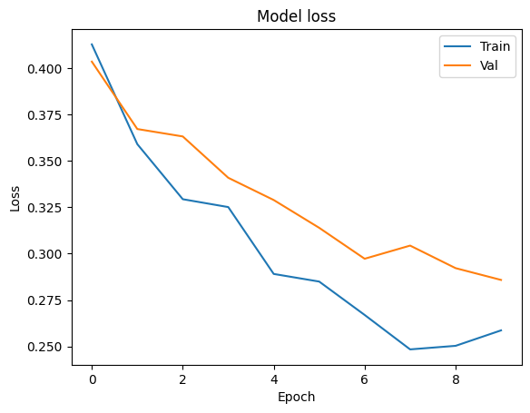
我们来可视化训练过程

[26]:

# Plot the change of loss during training
plt.plot(history['train_loss'])
plt.plot(history['val_loss'])
plt.title('Model loss')
plt.ylabel('Loss')
plt.xlabel('Epoch')
plt.legend(['Train', 'Val'], loc='upper right')
plt.show()

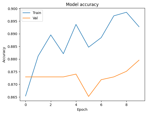
../_images/tutorial_Split_Learning_for_bank_marketing_62_0.png

[27]:

# Plot the change of accuracy during training
plt.plot(history['train_accuracy'])
plt.plot(history['val_accuracy'])
plt.title('Model accuracy')
plt.ylabel('Accuracy')
plt.xlabel('Epoch')
plt.legend(['Train', 'Val'], loc='upper left')
plt.show()

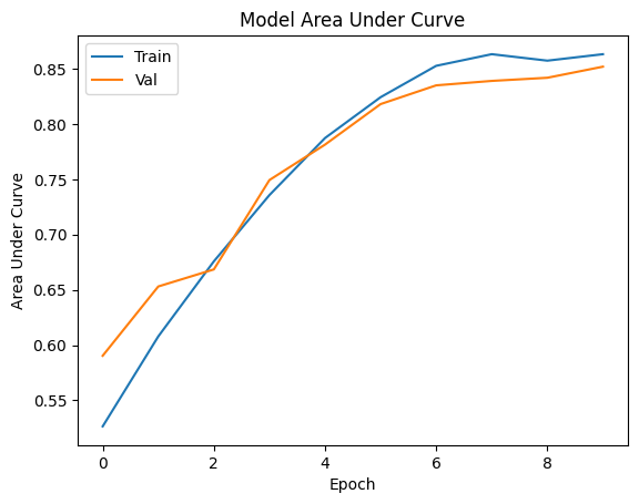
../_images/tutorial_Split_Learning_for_bank_marketing_63_0.png

[28]:

# Plot the Area Under Curve(AUC) of loss during training
plt.plot(history['train_auc_1'])
plt.plot(history['val_auc_1'])
plt.title('Model Area Under Curve')
plt.ylabel('Area Under Curve')
plt.xlabel('Epoch')
plt.legend(['Train', 'Val'], loc='upper left')
plt.show()

../_images/tutorial_Split_Learning_for_bank_marketing_64_0.png

我们来调用一下评估函数，看下训练效果怎么样

[29]:

global_metric = sl_model.evaluate(test_data, test_label, batch_size=128)

Evaluate Processing:: 100%|█████████████████████████████████████████████████████████████████████████████████████| 8/8 [00:00<00:00, 171.46it/s, loss:0.2899125814437866 accuracy:0.8751381039619446 auc_1:0.8452339172363281]

和单方模型的对比#

在这里，我们使用与分裂学习示例中相同的模型结构，但仅在这种情况下使用 Alice 的模型结构。定义模型的代码如下所示。
数据
数据也使用 Kaggle 的反欺诈数据集。在这里，我们只使用 Alice 的新银行数据。
样本量总计11162个，其中训练集8929， 测试集2233
2. The feature dimension is 4.

[30]:

from tensorflow import keras
from tensorflow.keras import layers
import tensorflow as tf
from sklearn.model_selection import train_test_split


def create_model():
    model = keras.Sequential(
        [
            keras.Input(shape=4),
            layers.Dense(100, activation="relu"),
            layers.Dense(64, activation='relu'),
            layers.Dense(64, activation='relu'),
            layers.Dense(1, activation='sigmoid'),
        ]
    )
    model.compile(
        loss='binary_crossentropy',
        optimizer='adam',
        metrics=["accuracy", tf.keras.metrics.AUC()],
    )
    return model


single_model = create_model()

数据处理

[31]:

import pandas as pd
from sklearn.model_selection import train_test_split
from sklearn.preprocessing import MinMaxScaler
from sklearn.preprocessing import LabelEncoder

encoder = LabelEncoder()
single_part_data = alice_data.copy()

single_part_data['job'] = encoder.fit_transform(alice_data['job'])
single_part_data['marital'] = encoder.fit_transform(alice_data['marital'])
single_part_data['education'] = encoder.fit_transform(alice_data['education'])
single_part_data['y'] = encoder.fit_transform(alice_data['y'])

[32]:

y = single_part_data['y']
alice_data = single_part_data.drop(columns=['y'], inplace=False)

[33]:

scaler = MinMaxScaler()
alice_data = scaler.fit_transform(alice_data)

[34]:

train_data, test_data = train_test_split(
    alice_data, train_size=0.8, random_state=random_state
)
train_label, test_label = train_test_split(y, train_size=0.8, random_state=random_state)

[35]:

alice_data.shape

[35]:

(4521, 4)

[36]:

single_model.fit(
    train_data,
    train_label,
    validation_data=(test_data, test_label),
    batch_size=128,
    epochs=10,
    shuffle=False,
)

Epoch 1/10
29/29 [==============================] - 1s 10ms/step - loss: 0.5564 - accuracy: 0.8261 - auc_3: 0.4520 - val_loss: 0.4089 - val_accuracy: 0.8729 - val_auc_3: 0.4384
Epoch 2/10
29/29 [==============================] - 0s 3ms/step - loss: 0.3771 - accuracy: 0.8877 - auc_3: 0.4524 - val_loss: 0.3969 - val_accuracy: 0.8729 - val_auc_3: 0.4322
Epoch 3/10
29/29 [==============================] - 0s 3ms/step - loss: 0.3653 - accuracy: 0.8877 - auc_3: 0.4417 - val_loss: 0.3911 - val_accuracy: 0.8729 - val_auc_3: 0.4316
Epoch 4/10
29/29 [==============================] - 0s 3ms/step - loss: 0.3601 - accuracy: 0.8877 - auc_3: 0.4514 - val_loss: 0.3875 - val_accuracy: 0.8729 - val_auc_3: 0.4443
Epoch 5/10
29/29 [==============================] - 0s 3ms/step - loss: 0.3585 - accuracy: 0.8877 - auc_3: 0.4626 - val_loss: 0.3855 - val_accuracy: 0.8729 - val_auc_3: 0.4680
Epoch 6/10
29/29 [==============================] - 0s 3ms/step - loss: 0.3571 - accuracy: 0.8877 - auc_3: 0.4737 - val_loss: 0.3839 - val_accuracy: 0.8729 - val_auc_3: 0.4867
Epoch 7/10
29/29 [==============================] - 0s 3ms/step - loss: 0.3557 - accuracy: 0.8877 - auc_3: 0.4879 - val_loss: 0.3828 - val_accuracy: 0.8729 - val_auc_3: 0.5052
Epoch 8/10
29/29 [==============================] - 0s 2ms/step - loss: 0.3547 - accuracy: 0.8877 - auc_3: 0.5001 - val_loss: 0.3818 - val_accuracy: 0.8729 - val_auc_3: 0.5164
Epoch 9/10
29/29 [==============================] - 0s 2ms/step - loss: 0.3539 - accuracy: 0.8877 - auc_3: 0.5107 - val_loss: 0.3807 - val_accuracy: 0.8729 - val_auc_3: 0.5290
Epoch 10/10
29/29 [==============================] - 0s 2ms/step - loss: 0.3530 - accuracy: 0.8877 - auc_3: 0.5212 - val_loss: 0.3799 - val_accuracy: 0.8729 - val_auc_3: 0.5368

[36]:

<keras.callbacks.History at 0x7fd7a85ec7c0>

[37]:

single_model.evaluate(test_data, test_label, batch_size=128)

8/8 [==============================] - 0s 1ms/step - loss: 0.3799 - accuracy: 0.8729 - auc_3: 0.5368

[37]:

[0.3799220025539398, 0.8729282021522522, 0.5367639064788818]

小结#

上面两个实验模拟了一个典型的垂直场景的训练问题，Alice和Bob拥有相同的样本群体，但每一方只有样本的一部分特征数据，如果Alice只用自己的一方数据来训练模型，能够得到一个准确率为0.583,auc 分数为0.53的模型，但是如果联合Bob的数据之后，可以获得一个准确率为0.893，auc分数为0.883的模型。

总结#

本篇教程，我们介绍了什么是拆分学习，以及如何在SecretFlow框架下进行拆分学习
从实验数据可以看出，拆分学习在扩充样本维度，通过联合多方训练提升模型效果方面有显著优势
本教程使用明文聚合来做演示，同时没有考虑隐藏层的泄露问题，SecretFlow提供了聚合层AggLayer，通过MPC,TEE,HE，以及DP等方式规避隐层明文传输泄露的问题。如果您感兴趣，可以看相关文档。
下一步，您可能想尝试不同的数据集，您需要先将数据集进行垂直切分，然后按照本教程的流程进行